Words don’t come easy (… to LLMs): Universal Text-Encoding for dynamic, multi-lingual alphabets revolutionizing efficiency and effectiveness for LLM training and inference

The remarkable advancements of Large Language Models (LLMs) frequently capture attention as they become valuable collaborators in daily situations, all while progressing towards breakthroughs beyond simple language completion. Beyond the standard tasks for chatbots that most offers can now solve reliably, the successful application to more specific problems and low-resource languages is still difficult to implement. This leads to questions of language fairness and domain specialization becoming crucial for a fair and scalable value creation. Still, the preferred industries’ solution for overcoming such challenges is the investment in even more compute – and construction of even larger models, ramping up costs and data needs to a point that is impossible for many cases. We developed an architecture innovation that addresses these points with a fundamentally different approach to text modelling.

Crucial initial steps for the construction of LLMs are tokenization, the discretization of text, and the embedding of resulting tokens into a numeric representation. In this blogpost we present a new paradigm for tokenization that significantly improves LLM training and inference and unlocks new capabilities for faster language-transfer of Large Language Models.

In short, we show that our innovation, “T-Free”, achieves

LLMs are a specific type of Artificial Neural Network trained on a massive corpus of text data. Training costs of a bigger, and as such more capable multi-billion parameter model easily exceeds several hundred million dollars (in 2024). The necessary acquisition and human labor investments further multiplies these. The first step in training these models is the conversion of natural language into a representation that the Large Language Model can process.

The core idea of transforming words into a machine-readable representation is surprisingly simple: We first build a dictionary, split the text by the rules of this dictionary into smaller chunks, called tokens[3], and map each token to a unique identification number (index in the dictionary). An example of the processing steps during a LLM prediction is shown in Fig.1. To build this dictionary, current approaches use statistical methods on a reference text corpus with the objective to reduce the total number of produced tokens on this corpus – while being constrained in the vocabulary size, i.e. the number of available tokens to choose from. The constraint is required as the vocabulary size directly influences the parameter number of the LLM.

In a way, this dictionary creation can already be regarded as a pre-training before the actual model training because the actual dictionary is solely dependent on the reference corpus that has been used, and remains fixed afterwards. Significant effort can be spent on optimization of the vocabulary –it afterall determines what the LLM is capable to comprehend– with the result only becoming apparent after a full model training.

Fig. 1 Processing Pipeline of LLMs: The input text is chunked by the tokenizer into unique numeric identifiers that the LLM processes to predict another such identifier — the next (sub-)word.

In Fig.1 above each word is represented by exactly one id. Most of the time, this is the ideal case, as we ensure that independent words get independent numbers and, as such, are independently trained from scratch. However, the vocabulary size is limited as it requires a trained parameter matrix in the LLM to convert the token numbers into processable state vectors. Therefore, we cannot encode entire words as they are, but need to re-use smaller parts for multiple words as much as possible. As an example, if the reference corpus did not include enough “common English language”, as it was (as usual) mostly accumulated from German websites, the phrase (underscore denotes whitespace):

“The_quick_brown_fox_jumps_over_the_lazy_dog.”

may be chunked into

“The”, “_qu”, “ick”, “_br”, “own”, “_f”, “o”, “x”, “_jump”, “s”, “_over”, “_the”,”_lazy”, “_dog”, “.”

with 15 tokens.

In this example, the token representation for “_jumps” is “_jump” and “s”. One might argue this is desirable, as a proper prefix was generated that can be reused to construct many continuing word variations such as “_jump”, “_jumps”, “_jumping” etc., while the full word stem remains the prefix.

Note, however, that whitespaces and capitalizations are explicitly encoded in the dictionary. Variations such as “the”, “The” and “_The” will be included as (almost) duplicates, exhausting the valuable vocabulary entries. They will get independent numbers assigned and as such will be trained independently from scratch, despite their close semantic meaning.

Furthermore, “quick”, “brown” and “fox” got split into multiple tokens, as well! This is the case whenever words were not frequent enough in the reference corpus the tokenizer was compiled with. The word “fox” got even split into 3 tokens, “_f”, “o”, and “x”. As such, the model needs to learn to reassemble these tokens into one word. Moreover, we require 3 times the processing effort to process – comprehend or predict – this split up word.

The purely statistical approach will also select strings that are an anomaly in the reference corpus and may not make sense with an objective view. In an older OpenAI tokenizer some tokens show this clearly, for example: ‘ SolidGoldMagikarp’, ‘_RandomRedditor’, ‘rawdownloadcloneembedreportprint’, ‘?????-?????-‘, ‘ÃÂÃÂÃÂÃÂÃÂÃÂÃÂÃÂ’, ‘ÃÂÃÂÃÂÃÂÃÂÃÂÃÂÃÂÃÂÃÂÃÂÃÂÃÂÃÂÃÂÃÂ’, ‘ TheNitrome’, ‘ TheNitromeFan’. It moreover has been demonstrated that use of these tokens results in errors, hallucinations, safety violations and mistakes in understanding related content[4].

Naturally, the more tokens a language requires for a given text, the less efficient the model performs on it, until it may not be able to comprehend it at all. The extreme case of letterwise tokens comes with a significant degradation in performance (compute demand and benchmark evaluations) and is still active research[5].

In summary, the LLM is trained to solve a high-dimensional pattern recognition task where every token is a completely new and independent dimension of the problem to be solved. Some words are split into multiple subwords as they were not sufficiently relevant when building the dictionary, while others appear multiple times, with only minor differences in typing characteristics. Both require specific skills of the LLM: The former to be able to merge word-splits and comprehend them together as one, the latter to identify near-duplicates and interpret them as the same. Flaws in the choice of vocabulary entries directly imply the maximal achievable language processing performance of the later trained LLM. The vocabulary is gathered solely based on statistics and matches by no means known scientific linguistical relevance. Once the model is trained, it is difficult to alter the vocabulary, e.g. when optimizing for use-cases like further specific language-capabilities or adding new languages.

The dictionary dictates the way a model interprets language and “thinks”. On an architecture level, it moreover influences the dimension of the first and last layer of a LLM, called Embedding and Head (we discuss them further below with Fig. 3 and 5). These, roughly speaking, convert the token-identification number into real number representations and back. For current state-of-the-art models, we use a bijective one-to-one mapping between these representations, and the corresponding matrices are of dimension vocabulary size x model hidden size. They are the largest occurring matrices in the language model, and as such significantly contribute to the total parameter count and computational (in-)efficiencies. Therefore they, and implicitly the dictionary, will be massively restricted. For models with “limited capabilities”, a vocabulary of 16k or 32k entries will suffice. However, in era of general-purpose all-rounder, recent state-of-the-art models contain a dictionary beyond 250k entries. These two layers then may sum up to 6B parameters[6] — only spent on converting token-ids to hidden states and back. This is 75% the size of an entire LLama3-8B, which can also process those.

As described, there is plenty of potential lost in the previously discussed classical approach.  In particular, we want to i) reduce the number of independently trained redundancies in the vocabulary ii) improve transfer learning between similar words and not learn everything from scratch as if there were no correlations between words and iii) allow flexibility for future use cases e.g. not drastically degenerate when continuing training with languages or word distributions initially not planned with. To this end we propose “Tokenizer-Free”, a new approach to encounter these Flaws. We show a comparison of the classical and T-Free approach in Fig. 3.

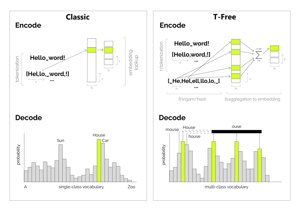
Fig. 3: Classic tokenizer with bijective vocabulary mapping (left) vs T-Free with multi-class vocabulary (right) for language text encoding (top) and decoding (bottom).

As a first step during encode (top-right), we split the input text by non-letters. As such we get exactly one embedding per word, no matter what spelling variation, which reflects more appropriately our natural experience. Since we now have many more possible words than entries in the embedding layer (for which we demonstrate that a vocabulary size v ≈ 16k suffices), we need to dissolve the bijective mapping between vocabulary and the embedding layer, which otherwise forces them to be of the same dimensions. As a solution we regard encodings of words as a mixture of w ≈ 50 random embeddings[7].

Naturally, as we now have a larger vocabulary than the embedding matrix, there will be overlaps in the patterns on the embedding layer. To bootstrap training and ensure proper language learning, we model a robust hash function between words, that ensures an overlap relative to the similarity, i.e. “more similar” words overlap more than others. As a measure for similarity, we employ a byte-based approach to ensure universality. Specifically, as shown in step 2, we build all character triplets of a word. In total there are n = wordlength such triplets, and we map each to m ≈ 10 embeddings. As a result, common stems or endings in words such as “jump” or “ing” will always be mapped to the same set of embedding activations. Furthermore, we enforce a 20% overlap of the activations with their lowercased variants. As such, arbitrary word capitalizations will at least share 20% of activations of the word written in lowercase. We found that these configurations accelerate the convergence of training and evaluation performance.

The final embedding, step 3, becomes the aggregation of all these, i.e. the sum of the entire active pattern with w = n x m entries.

Directly adapting the mentioned scheme, we also switch the models’ prediction objective from single- to multi-class. That means, instead of training the model to directly predict the particular vocabulary entry of the next word with a mono signal, we apply a training signal on the full w activations of the pattern of the next word. Arguably this may lead to a more robust training and recall behavior, as, again, single outliers may average out, and do not directly lead to devastatingly false word completions. In contrast to classical tokenizers, we again may find more similar words amongst the “highest” probable predictions as shown in the lower part of Fig. 3.

Our experiments demonstrate that we can reduce the embedding layer down to only 8k entries and still get improved model performance on most evaluations of an exhaustive benchmark suite, when comparing a 3B model pretraining with T-Free against a classical tokenizer training with a 64k vocab on the same data. A sweep on the required vocabulary size is shown in Fig. 4.

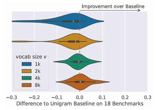
Fig. 4: Relative performance difference of a 3B T-Free model (8k vocab) to a 64k classical tokenizer. While a vocabulary size of 1k entries seems insufficient, T-Free’s clearly improves at a size of 8k.

This is a crucial step towards low-parameter models, that are in particular needed for the recent trend of deploying smaller LLM’s “on-the-edge”. In this experiment series we halved the total training cost[8]. As shown in Fig. 5, while the Parameter count can significantly be reduced, the averaged single-token inference time stays about the same due to the slightly more complex decoding strategy.

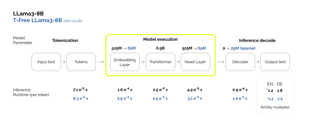
Fig 5: Parameter count and inference runtime comparison on LLama3-8B to a T-Free version (16k vocab).

Our word encoding is by design substantially different from that of classic tokenizers. In the following table 1 we demonstrate the large overlap of near-duplicates present in the vocabulary of classical tokenizers. Even though this vocabulary is essential to the model performance and its total parameter count, there is still little attention paid to optimization of the utilization of its vocabulary. By design our approach does not have explicit bijective entries that are only active for their vocabulary counterparts – and as such the embedding layer is fully utilized. We don’t have duplicates anymore. Moreover, words share synergies through spelling, and at least 20% of activations are shared amongst the same word, disregarding all writing capitalization variations.

Tab 1: Near-Duplicate statistics of prominent classical tokenizers and our proposed T-Free.

Furthermore, in Fig. 5, we demonstrate that the fertility —i.e. the average number of final embeddings required to represent a word— remains lowest for our proposed T-Free approach across languages. The performance of state-of-the-art tokenizers is heavily dependent on the distribution of the reference corpus. Languages underrepresented, as e.g. German or Russian in the baseline of the prominent LLama3, will result in higher fertility scores and as such decrease resulting model performance: Increased computation effort (i.e. required iterations) as well as reduced model comprehensive capabilities (as previously described).

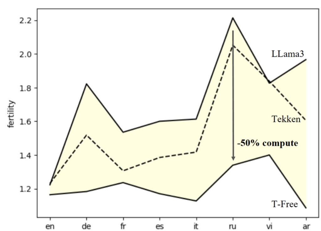
Fig 5: Fertility statistics (average encoding length per word) for various languages of state-of-the-art LLama3 and NeMo-Tekken tokenizers and our proposed T-Free.

Our proposed approach does not require a reference corpus and as such the resulting model is mostly unbiased w.r.t. its potential capabilities. This characteristic is usually referred to as “language-fairness”. T-Free achieves, even when comparing against large 256k entry vocabularies, up to 50% inference speedup on some languages through the lowered fertility scores. Visualized in Fig. 5 are scores of the recent LLama3 (128k; Meta) and NeMo-Tekken (131k; Mistral, Nvidia).

To demonstrate the impact of the previous statement, we conduct a transfer-learning experiment as follows: We train baseline models (with T-Free and classical Tokenization) mostly on English data, and afterwards continue training on mostly German data. In the following Fig. 6 we see differences in performances, averaged over several benchmarks: Out of the box T-Free, the left half, already performs (slightly) better on German data (orange). During continued training iterations, we observe that its performance rapidly increases on German, in particular when comparing to the classic approach. On top, the performance in English (blue) does not as drastically decrease – if at all – when comparing to the tokenizer approach that shows a clear downwards trend.

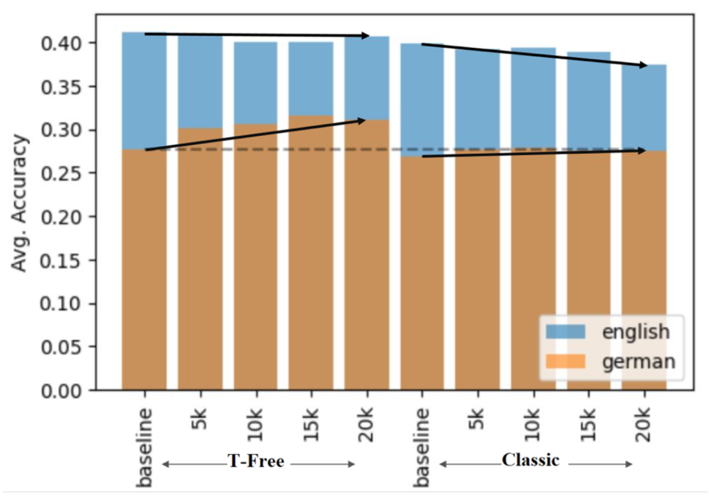
Fig. 6: Continued Pre-Training on an English/German data mix on models that were first trained on English only (“baseline”). T-Free shows better adoption to German, while retaining English performance. The classical Tokenizer, perhaps due to the differences in fertility, dropped performance in English, while slower adapting in German.

As part of our mission to accelerate and foster public research, we are committed to push reproducible code and models under open-aleph license, permissive for research and education.

Find the full research paper, code and model checkpoint here:
2406.19223 (arxiv.org), Aleph-Alpha/trigrams (github.com).

Shout out to all contributors, i.p. our collaborative team of researchers #Lab1141 at TU Darmstadt.

[1] As demonstrated on a 3B model configuration in the paper.

[2] Based on fertility metric comparison.

[3] The process of splitting text into tokens is referred to as “tokenization”, the entity as “tokenizer”.

[4] Source: https://www.lesswrong.com/posts/aPeJE8bSo6rAFoLqg/solidgoldmagikarp-plus-prompt-generation

[5] E.g. Charformer, T. Yi et al (https://arxiv.org/abs/2106.12672)

[6] Configuration of “command-R”.

[7] From combinatorics we can deduce that there are  such unique patterns.

[8] C.f. Fig. 4 of the paper.