Today, we are happy to announce the addition of Unit-Scaled Maximal Update Parametrization (u-μP) to Scaling, our official large scale training codebase. Together with Graphcore, we recently developed u-μP as a new paradigm to parametrize neural networks in terms of width and depth. Our approach combines μP, developed by G. Yang et.al., with Unit Scaling, a concept introduced by Graphcore.

The main benefits of u-μP are:

• A meaningful set of hyperparameters which transfer across model size and are easy to sweep.

• Stable numerical tensor scales during training, even allowing to perform the majority of linear layer matmuls natively in FP8 without any per-tensor-scaling strategy.

If you want to learn more details about u-μP, check out our paper.

We first give an overview about the theory behind u-μP and explain the main ideas. Then we give some practical tips and insights for people interested in using u-μP for LLM training.

To understand the very basic ideas and concepts behind u-μP, we start with the fundamentals.

The documentation of PyTorch’s nn.Linear, which is the module at the heart of most modern neural network architectures, states that weight and bias are initialized from the uniform distribution on [math](-1/\sqrt{\mathrm{fan\_in}}, 1/\sqrt{\mathrm{fan\_in}})[/math], where [math]\mathrm{fan\_in}[/math] is the number of input features to the layer. For notational convenience we abbreviate this by [math]d[/math]. There is a particular reason why [math]1/\sqrt{d}[/math] shows up here.

Let’s consider a freshly initialized linear layer [math]F[/math] with a weight [math]W[/math] (we assume no bias), and assume that the entries of [math]W[/math] are i.i.d with mean 0 and variance [math]\sigma_W^2[/math]. Now let [math]x[/math] be a random input with mean 0 and variance [math]\sigma_x[/math] that is drawn independently of [math]W[/math]. Let’s denote by [math]y[/math] the output of the layer, i.e. [math]y = F(x)[/math]. By assumption, the coordinate entries of [math]x[/math] are roughly of order [math]\sigma_x[/math]. But what about the entries of [math]y[/math]? By definition we have

[math]F(x)_i = \sum_{j=1}^{d} W_{ij}x_j[/math]

In modern deep learning, the hidden dimension d can get very large. Since the random variables [math]\{W_{ij} x_j \}_j[/math] are all independent and have mean 0 and variance [math]\sigma_W^2 \sigma_x^2[/math], we can apply the Central Limit Theorem (CLT) to deduce

[math]F(x)_i \sim N(0,\sigma_W^2 \sigma_x^2 d), \quad d \to \infty[/math]

Since we don’t want the hidden activations to shrink or grow too much when we change the network size, a good choice for [math]\sigma_W[/math] is one that is roughly proportional to [math]1/\sqrt{d}[/math], since then [math]y[/math] has a variance that is comparable to [math]x[/math] and is independent of [math]d[/math]. Another interesting observation is that [math]y[/math] becomes Gaussian in the limit, no matter what distributions [math]W[/math] and [math]x[/math] are drawn from, as long as all quantities are i.i.d and have finite variance, giving a hint why wide neural networks behave like Gaussian processes in the first forward pass.

While the analysis for a single linear layer forward pass is relatively easy, figuring out the correct scaling behavior for a whole neural network is a different beast, especially if one is interested in an analysis beyond the first forward and backward pass.

In a deep neural network, it is a priori unclear which tensors interact via the CLT and which tensors interact via the Law of Large Numbers (LLN) during training. The linear layer case above is an example where [math]W[/math] and [math]x[/math] interact via CLT in their matrix vector product because [math]W[/math] and [math]x[/math] are independent. As an example of a LLN interaction, consider the matrix [math]V = W \cdot W^T[/math] for some matrix [math]W[/math] with random i.i.d entries. The entries of [math]V[/math] are given by

Off the diagonal, the random variable [math]W_{ik} W_{jk}[/math] has mean zero, hence [math]V[/math] scales like [math]\sqrt{d}[/math] (CLT scaling). On the diagonal, we are summing [math]W_{ik}^2[/math] which has a mean of [math]\sigma_W^2[/math], hence those entries scale like [math]d[/math] by LLN.

During the first forward pass of a neural network, pretty much all tensors interact through CLT, but after one training step, the weights become correlated and the situation is less clear, especially with nonlinear operations involved. The above example of [math]W \cdot W^T[/math] is simple, but structurally this kind of correlated product actually occurs in subsequent forward passes when weights change through gradient-based updates.

In a major breakthrough, G. Yang et. al. fully analyzed the types of tensor interactions during training for very general types of networks called Tensor Programs. From this analysis, they deduced that there is a unique (modulo symmetry) way to parametrize the multipliers, initial variances and learning rates of the network weights by exponents of [math]d[/math] to guarantee maximal feature learning in the infinite-width limit. This parametrization is called Maximal Update Parametrization (μP).

To put it simply, the defining properties of μP are that neuron activations stay of order one during training, and all features (network hidden states for a given input) evolve non-trivially. The results of this work are significant because the class of Tensor Programs, for which the main theorems hold, contains a wide range of neural architectures, e.g. MLP, ResNet, Transformer, RNN. Furthermore, it was shown in Tensor Programs V that μP enables hyperparameter transfer from small to large models, a very valuable property that enables cost-efficient hyperparameter sweeps for LLMs.

While the main motivation of μP is establishing neural network dynamics with nice mathematical properties, it does not necessarily focus on numerical fidelity (more on this in the next section). With the goal of enabling stable FP8 training for neural networks, Blake et. al. from Graphcore introduced the concept of Unit Scaling in this paper. Unit scaling refers to the property that all tensors in a neural network (activations, weights and their gradients) have unit variance during initialization, i.e. the first forward and backward pass.

With high probability, entries of unit-scaled tensors naturally lie close to the center of the representable range of standard floating-point formats. This allows them to be cast to lower precision number formats like FP8. In practice, Unit Scaling is achieved in an inductive way. If we assume the input to a neural network to have unit variance, then the network satisfies Unit Scaling if every intermediate operation preserve this property.

In the linear layer example from above, we already calculated that the variance of the output y is given by [math]\sqrt{d} \cdot \sigma_W \cdot \sigma_x[/math]. Hence in order to preserve unit variance of an input ([math]\sigma_x = 1[/math]), the only choice is to set [math]\sigma_W = 1 / \sqrt{d}[/math]. The astute reader may protest here, and rightfully so. For Unit Scaling to hold, all tensors of the network need to have unit variance, but this is now violated by the choice of [math]\sigma_W[/math].

To resolve this problem, the crucial observation is that instead of changing the initialization of [math]W[/math], we can simply modify the linear operation itself: Instead of [math]F[/math], consider

Then this operation is scale preserving for [math]\sigma_W = 1[/math] if we set [math]\lambda = 1 / \sqrt{d}[/math]. This simple example already illustrates an important aspect of Unit Scaling. Due to the precise numerical constraint, weight multipliers like [math]\lambda[/math] are completely determined instead of being a hyperparameter of the model. We come back to this point later.

With the principle of Unit Scaling in mind, we now have to ensure that every operation, linear or nonlinear, preserves variance. Deriving analytical expressions for the scaling of all the common operations in Deep Learning can become quite involved, for a more in-depth look we refer to the Unit Scaling paper or this blogpost, which covers the scaled dot product operation specifically.

There are also a few more subtleties we want to mention. First, when shifting the scale from the initial variance of the weight to an op multiplier, the analysis does not change for a single forward pass, but the training dynamics change, since the multiplier also influences both gradients and weight updates (this is captured by abc-symmetry, see next section). Making a given network architecture unit-scaled while preserving its training dynamics is often possible but requires some care.

Second, we only considered the forward pass so far. In the backward pass of a linear layer, we multiply the incoming gradient with [math]W^T[/math] to get the gradient with respect to the input. But this means that if [math]\mathrm{fan\_in}[/math] is not equal to [math]\mathrm{fan\_out}[/math], the backward operation will not preserve variance. This can sometimes be resolved by utilizing the so-called cut-edge rule of Unit Scaling, but especially in residual networks this is not always possible. Another option is to interpolate between forward and backward scales as a compromise (which makes neither forward nor backward pass perfectly unit scaled), but we find that prioritizing Unit Scaling in the forward pass is usually the best practice.

Let’s quickly summarize what we learned so far.

μP is a method that

• aims to ensure nice mathematical properties of neural networks, leading to hyperparameter transfer.

• provides rules to scale weight multiplier, init variance and learning rate.

• guarantees activations stay of order one at each training step when increasing model width.

One of the practical drawbacks of μP is numerical stability. Tensor Programs V even reports that their 7B μP transformer model needed to be trained in FP32, which is very costly compared to lower-precision schemes.

Unit Scaling is a method that

• aims to ensure nice numerical properties of neural networks, leading to out-of-the-box low precision training.

• provides rules to scale weight multiplier, init variance (constant at 1) and nonlinear operations.

• guarantees that tensors have unit variance during the first forward and backward pass.

Unit Scaling focuses explicitly on numerics, but can only give guarantees at initialization. It does not give further recommendations on hyperparameters, especially learning rates and does not address tensor correlations during training. Given their conceptual similarities, it is natural to ask whether one can combine both approaches and get the best of both worlds while alleviating their respective blind spots. The answer is yes!

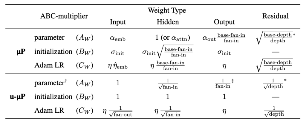
We found that there is a unique version of μP that satisfies Unit Scaling, which we call the Unit-Scaled Maximal Update Parametrization (u-μP). For people familiar with the scaling rules of μP it might look like Unit Scaling and μP are contradictory, since the hidden weight variance of μP is usually given by [math]1/\sqrt{d}[/math], whereas Unit Scaling requires a variance of 1. To resolve this, we have to talk about a fundamental property of neural networks (Lemma J.1 in Tensor Programs V) that we call abc-symmetry.

abc-symmetry states that the training dynamics (using the ADAM optimizer with [math]\epsilon=0[/math]) of any neural network are invariant under the following symmetry transformation:

where [math]A,B,C[/math] denote the multiplier, init std and learning rate and [math]\theta[/math] is any non-negative number. This statement can be proved in a few lines by application of the chain rule, but is the key tool to reconcile μP and Unit Scaling. Because of abc-symmetry, there is actually no unique μP but rather an infinite 1-parameter family of μP’s that are all equivalent. One can freely choose a scaling rule for either A,B or C which then determines the exponents of the other two. In case of Unit Scaling, we require that [math]B_W = 1[/math]. Then the unique version of μP satisfying this constraint is depicted in the following table:

Readers who are very familiar with μP will point out that our learning rate scaling rule is actually not in line with μP and they are right. During our transformer experiments we noticed that the optimal learning rate for the embedding matrix actually shifts quite a bit when increasing model width. Empirically we found that this shift is roughly given by an inverse square root law:

This finding is quite intriguing and we hope to give a theoretical explanation for this in future work.

Another thing to point out is the [math]1/d[/math] multiplier for the output weight. This rule actually violates Unit Scaling because the output logits tend to zero in the first forward pass as the width increases. We can live with that for two reasons: One, after the first model update, we know that the logits will be of order one. This behavior of the output layer is one of the main insights of μP and is caused by a change of tensor interaction (CLT vs. LLN) after the first forward pass. Second, since the output layer is the last operation before the loss calculation, the shrinking scale will not propagate to other layers. Enforcing Unit Scaling here by applying a [math]1/\sqrt{d}[/math] multiplier would lead to logits blowing up after the first step, which is a lot worse than violating Unit Scaling for this single layer.

On the other hand, the situation looks more dangerous for the backward pass, since here the magnitude propagates linearly through the network, underscaling every gradient along the way. Luckily, we can change the backward computation to apply the [math]1/\sqrt{d}[/math] factor in the backward pass. Even though this produces a mathematically “wrong” gradient, the error is just a constant factor which is pretty much ignored when using ADAM, or can be compensated for in the optimizer when using SGD (akin to loss scaling).

To summarize:

• Unit Scaling dictates a constant scaling for the init std of model weights. We use abc-symmetry to identify the unique version of μP that satisfies this constraint.

• Empirically we identify a better rule for the embedding learning rate in transformer models.

• We apply a manual scale correction in the input gradient calculation of the output layer, applying [math]1/\sqrt{d}[/math] instead of [math]1/d[/math] to restore Unit Scaling in the backward pass.

Observe that the Unit Scaling condition also removes the global init std gain parameter that is a commonly used hyperparameter of μP. One could ask whether the removal of hyperparameters is too restrictive, leading to the risk of being in a bad region in hyperparameter space. We address this question next.

With weight multipliers and initial variance removed from the hyperparameters, at a first glance it looks like we have heavily restricted the hyperparameter space. Individual learning rate multipliers are still admissible, although empirically we find that tying those to a global learning rate usually works well.

To ensure enough expressivity in our parametrization, the crucial observation is that we can actually re-introduce multipliers in certain parts of the model where scale does not propagate. Let’s illustrate this with an example. Consider the FFN of a transformer block:

where [math] F_{down}[/math] and [math]F_{up}[/math] are the linear projections without bias and [math]\varphi[/math] is the non-linearity. Usually there is a skip connection around the FFN, so the actual output is calculated as

Remember that every linear layer comes with a fixed multiplier that guarantees Unit Scaling. Let’s assume we want to change the multipliers associated with

[math]W_{up}[/math] and [math]W_{down}[/math] by factors [math]\alpha_{up}[/math], [math]\alpha_{down}[/math] respectively. We can implement [math]\alpha_{down}[/math] by simply introducing a new activation function [math]\varphi_\alpha(x) = \varphi(\alpha \cdot x)[/math]. This works because the linear operation propagates the factor [math]\alpha_{down}[/math] to the next operation. If [math]\varphi = \mathrm{GeLU}[/math], then [math]\varphi[/math] does not propagate the scale and we get a proper new hyperparameter in form of the pre-activation temperature for the GeLU function. For [math]\alpha_{up}[/math], we can actually define a scaled residual add operation with a residual gain parameter

and subsume [math]\alpha_{up}[/math] in the residual gain.

If [math]\varphi = \mathrm{ReLU}[/math], then [math]\alpha_{down}[/math] can actually be propagated further to the next linear operation and directly to the residual add operation. In this case we don’t get a temperature for the activation function and subsume both weight multipliers in the residual gain parameter of this residual block.

In general, residual add operations and non-homogeneous operations (like softmax or GeLU) do not propagate scale and introduce a multiplier that is associated with this operation, rather than being attached to a specific weight. Of course, by introducing temperatures for these nonlinear functions we skew the variance of the output and have to adjust the post-op scaling factor to restore Unit Scaling. For residual add operations this becomes even more involved and requires an additional trick. Going into this is out of scope for this blogpost, but we refer the interested reader to the appendix of our paper, where this is explained in detail.

Following this procedure through the whole pre-norm transformer architecture, we identify 5 meaningful hyperparameters, which we call u-multipliers:

1. The pre-attention-softmax temperature [math]\alpha_{attn-softmax}[/math].

2. The pre-nonlinearity temperature in the FFN [math]\alpha_{ffn-act}[/math], assuming standard GeLU or SwiGLU FFN.

3. The attention residual gain [math]\alpha_{res-attn}[/math].

4. The FFN residual gain [math]\alpha_{res-ffn}[/math].

5. The pre-loss-softmax temperature [math]\alpha_{loss-softmax}[/math].

We actually found it beneficial for hyperparameter independence to re-parametrize the residual gain factors into two new hyperparameters:

• [math]\alpha_{res}[/math] which is the overall residual strength.

• [math]\alpha_{res-attn-ratio}[/math], which controls the contribution of the attention residual relative to the FFN residual.

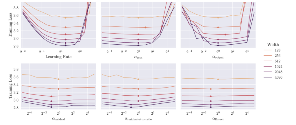
We find these canonical multipliers to be fairly independent, which makes hyperparameter sweeps much easier. Instead of a costly grid or random search, simply sweeping one of our hyperparameters after the other leads to the same downstream loss after considerably fewer trials.

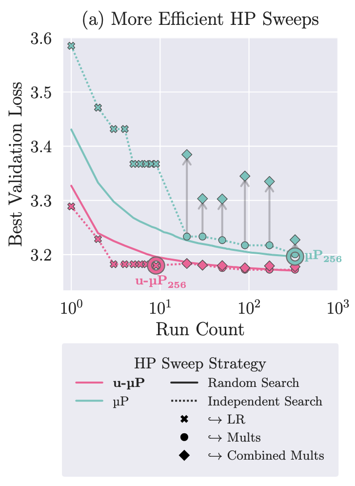
Moreover, global learning rate and u-multipliers all transfer well across model size, with their default value of 1 for the u-multipliers often close to optimal.

As a final remark, we want to stress that using our u-multipliers and potentially individual learning rates for some parameter groups, u-μP can represent almost any hyperparameter configuration at a given model size. Similarly to how we devised u-μP in the first place, one has to use abc-symmetry to shift all weight variances to 1, then absorb all resulting weight multipliers in our u-multipliers. This takes a bit of practice to do, but the reward for anyone who is already happy with their model hyperparameters is that they can translate these into u-μP to profit from the benefits, like an out-of-the-box partial FP8 training scheme (see next section).

We conclude with a training report of u-μP in a realistic training scenario. This should serve as a good starting point for anyone interested in applying u-μP for LLM training.

Architecture. We use a more or less standard transformer architecture fashioned after LLAMA 2:

• Pre-norm residuals

• SwiGLU FFN

• No biases

• RMS norm (non-parametric)

• No weight tying

• No group query attention

• No QK norm

• No gradient clipping

• No z-loss

• 4M token batch size (4096 sequence length and 1024 batch size)

• We don’t reset the attention mask between documents

• Cosine lr schedule decaying to 10% of max lr, 500 warmup steps

• Independent weight decay of [math]2^{-13}[/math]

• No dropout

• Rotary positional embeddings with base 1e4

• Head dimension of 128

The independent weight decay, non-parametric norms and absence of biases are choices we highly encourage when using u-μP, judging from our experiments.

We deliberately omit what we consider ad-hoc stabilization techniques like QK normalization, gradient clipping and z-loss because u-μP was specifically designed to facilitate stable numerics. One can still apply those (although gradient clipping would need to be adjusted to gradient sizes of order one), but with u-μP they might not be necessary anymore.

We scale number of layers and number of attention heads (using as many heads as number of layers) from 16 to 24 to 32, arriving at models with roughly 1B, 3B and 7B parameters.

We train for 72k iterations (~300B tokens) on the SlimPajama dataset.

For the learning rate and u-multipliers, we perform an independent sweep on a small proxy model and find the following optimal values:

• learning rate [math]\eta = 2^{3.5}[/math]

• attention residual ratio [math]\alpha_{attn-residual-ratio} = 2^{-2}[/math]

• all other multipliers are kept at 1.

The learning rate and attention residual ratio had by far the biggest impact during our sweeps, so we recommend to at least optimize those two.

FP8 mixed precision. In initial training runs, we tracked the magnitude of tensors throughout the model. Most tensor scales stabilize and do not grow significantly larger than their initial scale of 1. However, the input tensors to the attention dense projection and the final FFN projection (we call these operations critical matmuls) exhibit sudden explosive growth in some layers:

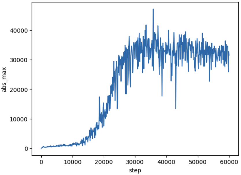
This might be related to the formation of outlier features (see this paper) and warrants future investigation.

Based on these observations we trained models with the following FP8 mixed precision scheme:

• We cast the input and the weight of non-critical matmuls to FP8 E4M3 and the gradient w.r.t. the output to FP8 E5M2.

• Critical matmuls, embedding and decoder head stay in BF16.

• Optimizer states stay in FP32.

The difference between E4M3 and E5M2 is that the first uses 4 bits to represent the exponent and 3 bits bits to represent the mantissa whereas the latter uses 5 bits for the exponent and 2 bits for the mantissa. For more information we refer to this paper.

We emphasize that we do not perform any kind of ad-hoc per-tensor-scaling, as is usually the case in FP8 training. Because of the well-behaved numerical scales we can simply cast to FP8 (note that one could still use per-tensor-scaling if desired, we just demonstrate that it is not required for a majority of tensors when using u-μP).

With this partial FP8 scheme, roughly 70% of matmuls in the transformer layer are performed in FP8, directly leading to a 35% decrease in memory footprint of the model weights during inference. As for throughput, in theory, FP8 matmuls on Nvidia H100 hardware can be performed twice as fast as their 16 bit counterpart. However, fully tapping into this potential requires technical optimizations that were out of scope for this paper. We plan to explore this and other potential FP8-related speedups during training in future work.

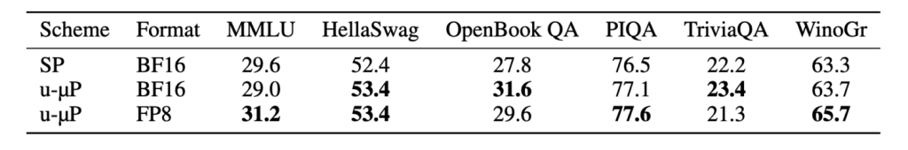
To test both the fidelity of our FP8 mixed precision scheme as well as our hyperparameters we trained two further baselines alongside our u-μP FP8 models:

• u-μP in standard BF16 mixed precision

• A standard parametrization (SP) baseline which uses the depth-scaled initialization scheme from Pythia and a learning rate scheme that scales inversely linear with hidden size (6e-4, 4e-4, 3e-4).

The results of these trainings is depicted below:

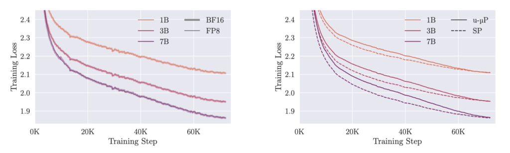
We see that the FP8 models closely match the loss of their BF16 equivalent. As for u-μP vs SP, we see that the two model families have quite a different optimization trajectories, with SP having a lower loss in the beginning of training, but u-μP catching up towards the end. Downstream evaluations complete the picture and show almost no degradation of the FP8 models and an overall strong performance of u-μP.

Topics like infinite-width-limits, hyperparameters and numerics can be quite challenging for the uninitiated, and u-μP touches upon all of those. We hope that readers who are completely new to these areas as well as more experienced folks learned a thing or two from this blogpost and are now eager to dive deeper into our work and that of our predecessors.

While u-μP marks a milestone for us and hopefully others, there are still many open questions. We still lack a unified understanding of the training dynamics of neural networks, which makes empirical hyperparameter search a necessity in the first place. On the side of low-precision training and efficiency, we firmly believe that model design choices that are founded on mathematical principles like u-μP can facilitate further optimizations and push model performance.

To learn more about u-μP, feel free to check out our paper. If you are interested to experience u-μP in practice, you can find our code on Github and the model checkpoints in our Huggingface repository.