






Eric Schreiber
Inference Performance from First Principles
TL;DR: What limits inference speed depends on the serving scenario, where multiple interacting factors can become the bottleneck. Reasoning about these bottlenecks from first principles is tedious by hand, so we built an analytical model to do it for us. This post uses it to build a mental model of what matters for fast inference.
Introduction
Training a transformer is a one-time cost. Serving it is not. Every request a model handles in production requires a forward pass, and at scale the cumulative cost of inference is significant. Yet inference performance is rarely taught alongside the architecture itself and it turns out to be surprisingly nuanced.
It depends strongly on model architecture and deployment strategy, and their interactions make it difficult to isolate what drives performance in a given setting. To reason about this systematically, we built CHEETAH, an analytical model that estimates inference performance from first principles. It decomposes each forward pass into the three main bottlenecks of an accelerator: compute, memory movement, and communication. Given a model architecture, hardware specifications, and a parallelism strategy, it produces an upper-bound estimate of achievable inference speed.
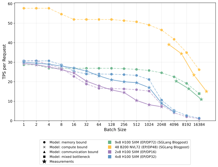
Figure 1 shows that once calibrated, CHEETAH tracks measured throughput across batch sizes spanning three orders of magnitude and, more importantly, correctly predicts where the bottleneck shifts. The full formulation and validation of CHEETAH are in the appendix.
The rest of this post uses CHEETAH to reason from first principles and build an understanding of what limits inference speed. We examine both inference stages, prefill (processing the input prompt) and decode (generating the output tokens one by one), separately as each is governed by a different bottleneck. We start with analysing dense models, specifically the widely studied Llama 3.1 70B, before turning to MoE architectures, and close with a brief look at how the field's focus has evolved.
What matters for fast inference?
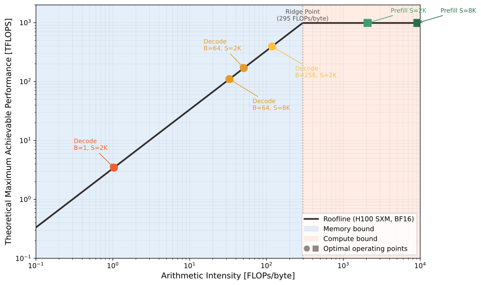
As mentioned above, inference can be divided into two stages: prefill and decode. Both of these stages map to important customer-facing metrics: time to first token (TTFT) and inter-token latency (ITL). TTFT is how long a user waits before the first token appears, while ITL, or its inverse tokens per second (TPS), measures how quickly tokens stream out during decode. We will examine both phases in more detail in the next two subsections. But at a high level, prefill is compute-bound, meaning that the FLOP throughput of your accelerator (how many floating-point operations it can execute per second) largely determines performance. On the other hand, decode is memory-bound, with inference speed primarily dictated by how much data must be loaded from memory for each generated token and the memory bandwidth available on the accelerator.
The roofline plot1 in Figure 2 visualises this nicely. During prefill the arithmetic intensity is high, meaning we perform many FLOPs per byte loaded, because we have large matrix-matrix multiplications, and the operation hits the compute ceiling. During decode, arithmetic intensity is extremely low and we sit deep in the memory-bound region. Performance is therefore limited by how quickly data can be moved from memory to registers, leaving much of the available compute underutilised. This is mostly because during decode we generate one token at a time and thus have matrix-vector (or matrix-thin_matrix) multiplications, instead of efficient large matrix-matrix multiplications, reducing the reuse of loaded data (e.g. the model weights).2
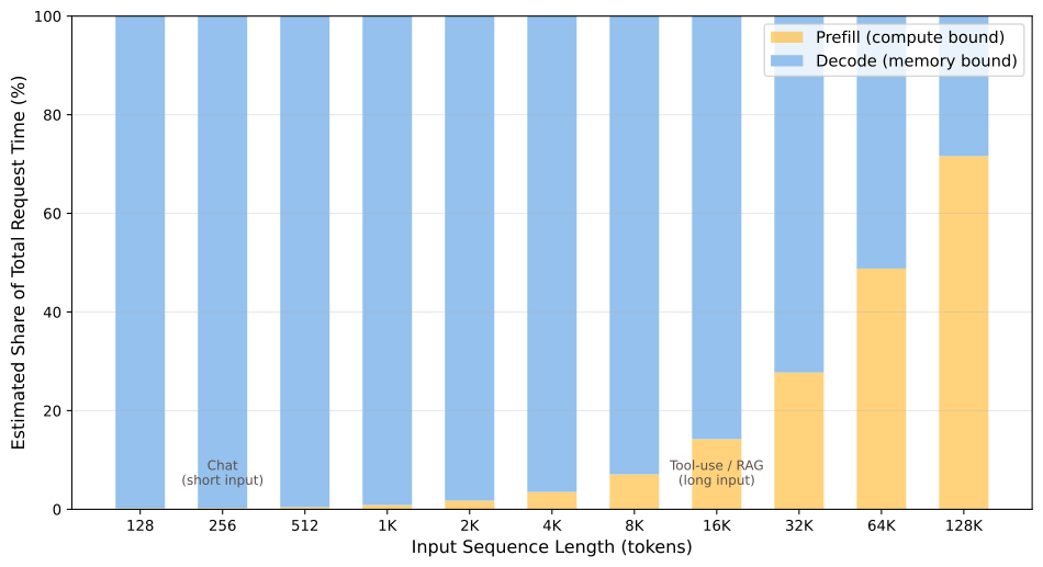
The balance between time spent in prefill vs decode depends heavily on the use case. Figure 3 shows how the split changes with input length: decode time dominates chat scenarios (short inputs, long outputs), while scenarios with long inputs (such as tool-use or Retrieval-Augmented Generation (RAG) workflows) spend a significant fraction in prefill.3
Prefill
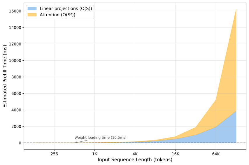
The prefill phase processes the entire input prompt in a single forward pass.4 This makes it possible to process the whole sequence as large matrix-matrix multiplications. This means each weight matrix is loaded from memory once and reused across every token in the prompt; the number of operations per byte, we call this the arithmetic intensity, is high. The compute required scales as for the linear projections (Q, K, V, O, MLP) and as for the attention ( and ). At short sequences the linear projections dominate; at long sequences the quadratic attention component takes over (Figure 4).
What matters for prefill performance:
- FLOPs of the model: Since we are compute-bound, the number of floating-point operations directly determines the time to first token (TTFT; the metric we care about during prefill). Fewer attention heads, smaller hidden dimensions, or sparse attention patterns all reduce TTFT.
- Sequence length: Attention compute scales quadratically. This is why sparse and linear attention mechanisms are being actively researched (e.g. linear attention, Mamba, GDN, DSA, MSA, and more).
- GPU compute throughput: Unlike decode, prefill benefits directly from higher FLOP throughput (e.g. using numeric precisions that run more operations per second, or simply faster hardware).
Prefill is relatively "easy" to make efficient: we have large matrix multiplications that fully utilise the GPU's tensor cores5. The challenge is keeping the TTFT acceptably low at long context lengths, where the quadratic attention cost dominates. This motivates self-attention mechanisms that have sub-quadratic scaling.
Be cautious with average TTFT numbers
An interesting observation is that the globally tracked TTFT can be influenced by how the inference engine6 schedules its prefilling requests. Consider a scenario with identical incoming prefill tasks, each of sufficient length. Prefilling a single task takes . Since we are compute-bound as established above, we can assume that batching scales time linearly with batch size as every task requires the same number of FLOPs.
Consider two scheduling strategies: (1) prefill the entire batch simultaneously, so every request receives the same TTFT, or (2) process all tasks one after another, giving some requests better TTFT than others. Looking at average TTFT alone, for :
Clearly for any batched inference setting. The schedule that minimises the average TTFT does so by spreading individual TTFTs unevenly, with the first request being served immediately while the last waits the full . Batching, by contrast, equalises TTFTs across all requests but at the worst-case value. In practice, this effect is less pronounced in continuous serving scenarios where requests arrive at different times and are therefore in different processing states.
Finally, note that the linear scaling assumption is an approximation, so the gap between the two scenarios is narrower in practice than the expressions above suggest. The qualitative argument, however, remains valid.
All of this shows why an inference provider should care about the full TTFT distribution and not just its mean.
Decode
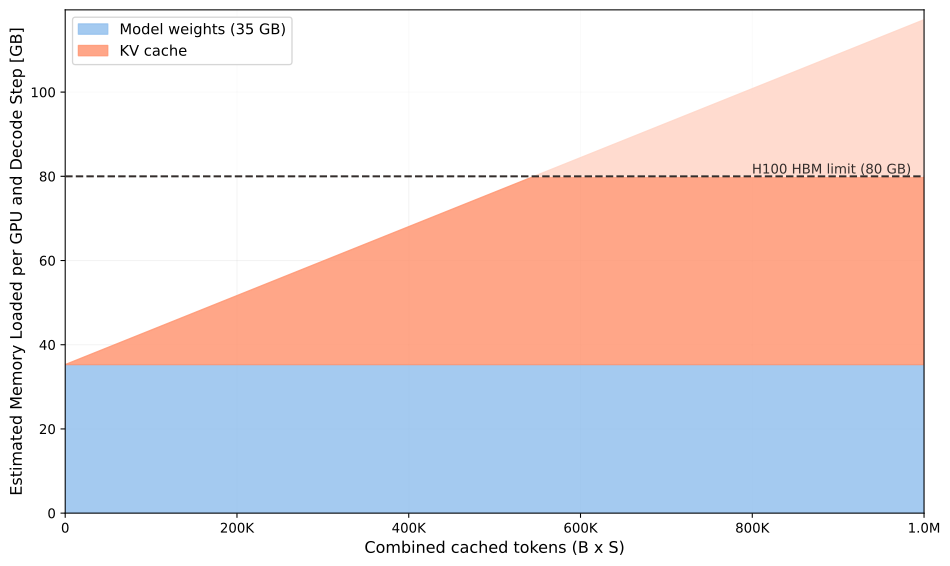
Decode generates tokens one at a time. Each step requires loading the full model weights from memory but performs relatively little computation per loaded byte, meaning the arithmetic intensity during decode is lower than that of the hardware. This makes decode fundamentally memory-bandwidth-bound in most practical scenarios. The time per decode step is approximately:
Figure 5 shows this visually for Llama 3.1 70B. The MLP weights and attention projection weights form a fixed-cost floor that must be paid every single decode step but can be amortised over the batch size. The KV cache adds a variable component that grows linearly with the number of cached tokens (batch size × sequence length).
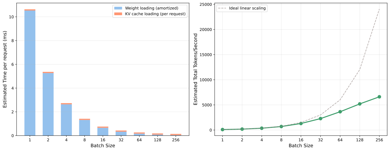
The key insight for decode economics is batch amortisation: since loading weights is the dominant fixed cost, serving multiple requests simultaneously, turning many sequential matrix-vector multiplications into a single large matrix-matrix multiplication, shares that cost across all of them, because the weights are loaded only once for the whole batch. This is visualised in Figure 6. The trade-off is latency: each request's KV cache is still loaded every step and is not shared. As the batch grows the ITL seen by any individual user rises. Batching therefore trades per-request latency for throughput. The model provider's goal is to maximise throughput, given this constraint of a minimal per-request TPS.
However, decode is not uniformly memory-bound across all operating points. The bottleneck type shifts depending on the batch size and sequence length. We can map this onto four qualitatively different regimes (Figure 7):
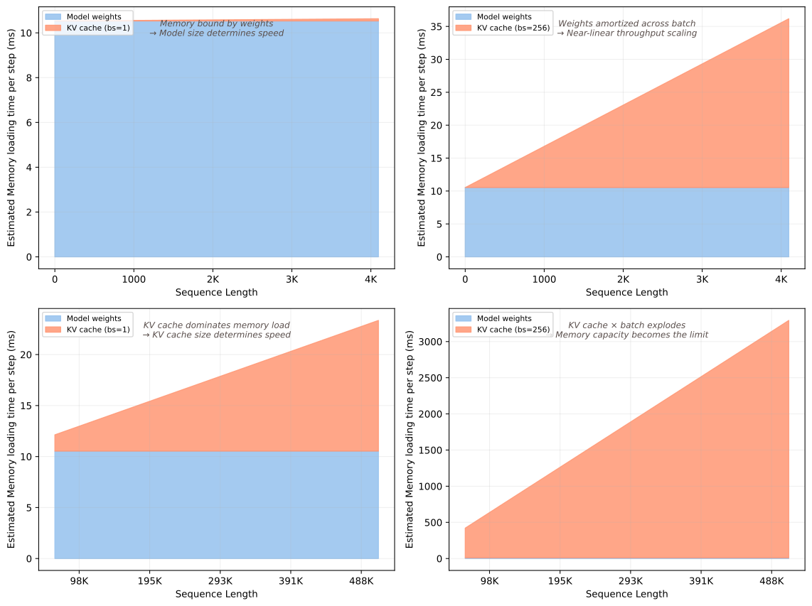
Low batch size, short sequence length
- Firmly memory-bound; model size (total parameter count × bytes per parameter) directly determines TPS
- KV cache is negligible compared to model weights
- Per-request TPS is near peak (you are in the regime of minimal memory movement)
- Optimisation lever: quantising to lower precisions (FP8 or INT4) to reduce weight size
High batch size, short sequence length
- Weight loading is amortised across many requests → higher total throughput, more efficient system but lower per-request TPS
- Can approach compute-bound regime at very large batch sizes
- Showcases the goal of inference: maximise throughput while still meeting minimal per-request TPS
- Memory footprint and per-request TPS constrain maximum batch size
- Optimisation lever: you are in the most efficient regime. To run faster you can scale out, parallelising over more GPUs
Low batch size, long sequence length
- KV cache loading dominates the per-step time (can exceed weight loading at long contexts)
- Memory-bound, but now by KV cache rather than weights
- Per-request TPS degrades linearly with sequence length
- Optimisation lever: KV cache compression (GQA/MLA/HCA), quantised KV cache, sparse attention patterns that skip loading parts of the cache (e.g. DSA and others)
High batch size, long sequence length
- Both KV cache and attention compute are large
- GPU memory is the hard constraint: storing the KV cache for many long sequences exhausts memory, forcing evictions and reducing effective batch size
- Optimisation lever: multi-node serving (more memory), KV cache offloading from memory to disk, prefill-decode disaggregation7, dedicated long-context nodes
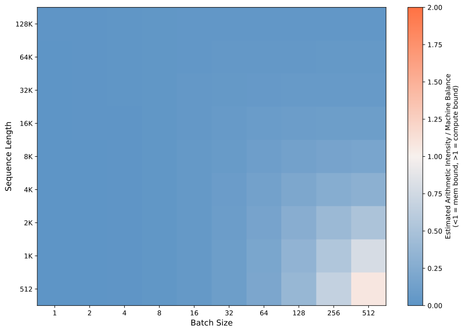
In summary, we can plot the aggregate arithmetic intensity of an inference against the machine's balance to show how close we can get to the compute-bound regime during inference for different scenarios in Figure 8.
What changes for MoE models?
The analysis above assumes dense models because they are simpler to reason about, but Mixture-of-Experts (MoE) architectures have clearly become the standard and shift the picture in a few ways. Unlike a dense model, where every parameter is used for every token, an MoE model activates only a small subset of its total parameters (in granularity called experts) per token at each layer. As a result, the per-token FLOPs are much lower than the total parameter count would suggest. This sparsity is what lets MoE models grow so large, which in turn pushes you towards bigger multi-GPU setups just to hold the weights in memory.
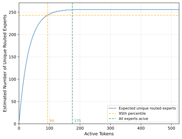
That sparsity also changes which regime you land in. Each individual expert's MLP is small, and applying TP sharding results in the weight matrices getting too narrow to saturate GPU tensor cores. The natural solution is Expert Parallel (EP) sharding, where different experts live on different GPUs. With each expert only seeing the fraction of the batch routed to it (Figure 9), the per-expert batch size stays smaller for longer, so you need a much larger batch than with dense models for the model to get close to the compute-bound regime.
Additionally, EP requires routing tokens to the GPU that holds the selected expert, introducing an all-to-all communication step every layer. At large batch sizes nearly all experts get activated across the batch, so every GPU must exchange tokens with every other GPU. This communication overhead can become the dominant bottleneck, making MoE decode sometimes even communication-bound, which has the potential to be even slower than memory-bound.
Prefill or decode: what to optimise for
Historically, most attention was focused on training efficiency. As a result, model architectures were typically compared on a FLOP-matched basis, which is still a good proxy for accuracy but not for inference speed. More recently, the field began shifting towards inference-efficient architectures, with much of the focus placed on improving decode efficiency. The reason is economic: a model is trained once but then served to many users over its lifetime, so the one-time training cost, however large, is eventually dwarfed by the cumulative cost of inference.
That emphasis is now evolving again. With architectures such as DeepSeek v4, it seems that frontier labs are increasingly considering both prefill and decode performance rather than optimising exclusively for decode. Why the renewed interest in prefill? One likely reason is the growing prevalence of tool use and RAG workflows. These systems often introduce large amounts of context that must be processed before generation can begin, increasing the amount of work performed during prefill. As a result, the time spent in prefill and decode becomes more balanced than in a typical chat interaction. The widespread use of speculative decoding8 has contributed to the same effect.
What this trajectory illustrates is that the right optimisation target is not fixed. As serving patterns shift, so does the bottleneck. That is precisely why first-principles reasoning matters: rather than optimising for one metric, understanding what an accelerator is actually doing, and thus the current bottleneck, makes it possible to anticipate where the next constraint will appear.
Appendix: CHEETAH
CHEETAH — Compute Heuristics for Estimating Execution Time And throughput on given Hardware.
Inference performance is impacted by many interacting factors, and it is hard to reason about all details a single change affects. Change the attention mechanism, optimise the parallelism strategy, and check if the workload on an accelerator is compute-, memory- or communication-bound, doing this all by hand is tedious and error-prone. CHEETAH is an attempt to reason about these bottlenecks from first principles and to iterate on them with a fast response time. It reduces an architecture, parallelism strategy, and hardware to a handful of parameters that can be compared before committing to an implementation.
The predicted absolute numbers should be read as a theoretical speed ceiling, not a throughput you will achieve in practice. What CHEETAH gets right is the structure: where the bottlenecks are, and how architectures and setups rank against one another. Given good implementations and hardware alignment, that ranking is invariant, which is what makes the model useful for design-space exploration.
This appendix describes CHEETAH's design, formulation, limitations, and validation.
What CHEETAH models
CHEETAH estimates the time for a single forward pass by computing per-layer contributions from four potential bottlenecks:
- GPU computation time: based on FLOPs per layer and hardware peak throughput.
- GPU memory movement time: based on bytes loaded from HBM per layer and hardware memory bandwidth.
- Inter-GPU communication time: based on the collective (all-reduce, all-gather, all-to-all), communication volume, interconnect bandwidth and network topology.
- CPU overhead: fixed per-layer kernel launch overhead plus global per-forward-pass overheads.
For each layer component the memory and compute times are
where is bytes loaded from HBM, is FLOPs, and and are the hardware's memory bandwidth and peak FLOPs. The factors capture the gap between theoretical peak and what kernels actually achieve: the cache misses, occupancy limits and implementation inefficiencies that keep real performance below the roofline.
Communication time depends on the type of collective operation and the actual algorithmic implementation we use,
with data volume , interconnect bandwidth , and an algorithm-dependent factor for GPUs:
| Algorithm | All-Reduce | All-Gather |
|---|---|---|
| Ring | ||
| Tree | — | |
| Butterfly | — |
To model multi-node setups with heterogeneous networks (unidirectional NVLink intra-node GB/s; InfiniBand inter-node GB/s9), CHEETAH optionally models the bottleneck of the full network:
Depending on the sharding used, communication is either overlapped or applied in series,
The full forward pass sums the layers and adds the CPU overheads on top,
where is per-layer kernel-launch overhead, is global scheduling overhead, and is a batch-size-dependent static overhead. From we derive the throughput and latency metrics used throughout the post. Usually these static overheads can be ignored. For small models (under 1B parameters), however, they become significant.
Parallelism defines how the work is divided on the hardware. Tensor parallelism splits weight matrices across GPUs, so FLOPs and memory scale as at the cost of an all-reduce after the row-parallel layers. Data parallelism replicates the weights and splits the batch, with no communication during inference. Expert parallelism distributes the experts of an MoE across GPUs and uses an all-to-all to dispatch and combine tokens. Combinations of the three are supported.
CHEETAH also calculates the largest batch that fits, bounded by global memory size
with GPU memory , model weight memory , and per-sequence memory (KV cache plus activations). If the requested batch exceeds , CHEETAH either runs at the reduced size or issues a warning.
Limitations and assumptions
CHEETAH is a theoretical model, and while modelling the major bottlenecks encountered during inference, it still needs to make certain assumptions. It assumes steady state (meaning a fixed batch size and sequence length), and so does not model continuous-batching dynamics as requests arrive and leave (non-trivial, especially for prefill), variable sequence lengths within a batch, or prefill-decode interference when the two are co-located. The inefficiency factors are calibrated once from measurements and then held constant to avoid overfitting on the measurements, even though real efficiency drifts with batch size and sequence length. We use separate for attention versus MLP and for memory, compute and communication, but they remain approximations. Communication is modelled as purely bandwidth-limited, so latency-bound communication cases, as can sometimes be encountered with small models, are not captured.
Validation
To validate CHEETAH, we gathered measurements on the inference performance of DeepSeek v3 and calibrated the inefficiency factors once per model (keeping them constant over all different setups), anchored on known kernel characteristics where these are public (FlashMLA reaching about 0.66 MFU, DeepGEMM around 1550 of 1980 TFLOPs, DeepEP around 40 GB/s over InfiniBand with higher bandwidth over mixed networks) and optimised with Bayesian optimisation. We reuse the same inefficiency factors across all batch sizes and inference setup configurations (different parallelisation and hardware setups) for the same model.
DeepSeek v3 tests most of CHEETAH well: it is MoE, it runs at large scale (meaning its static overheads are small, thus a steady-state model has more accurate predictions), and it has a lot of publicly available inference performance numbers, more than almost any other open model. We compare against measurements we generated ourselves for the smaller setups (2 and 4 nodes of H100 SXM, using SGLang with DeepEP and DeepGEMM; setup instructions) and against published SGLang numbers for the large-scale setups (large-scale EP, GB200 NVL72).
Figure 1 at the top of this post shows the per-request throughput across this range; Figure 10 breaks the same comparison down per GPU to show the different efficiencies achievable with the different setups.
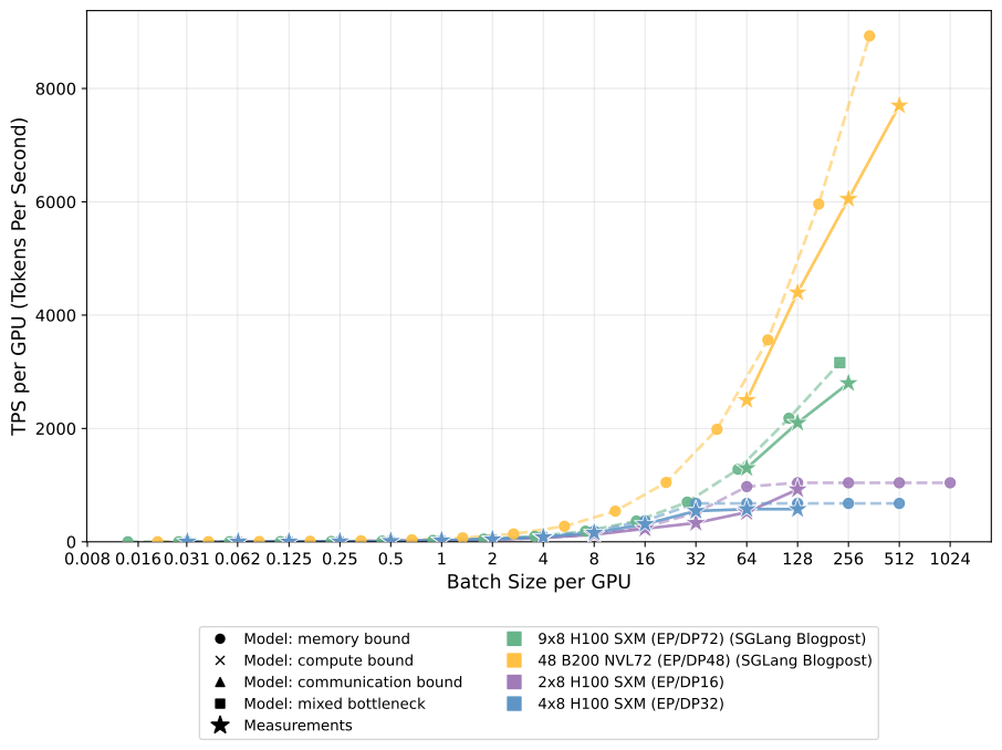
Across this range CHEETAH tracks the measured trend and, just as importantly, predicts where the bottleneck moves. That is what makes it useful for the design-space sweeps in this post: the absolute numbers are estimates, which show the theoretical speed ceiling. But the relative comparisons between architectures and setups are consistently ranked.
Acknowledgements
A special thanks goes to Piotr Mazurek. Looking at inference bottlenecks from first principles was Piotr's idea, and this work derives from what we did together for the DeepSeek Inference Theoretical Model at Aleph Alpha. Many of the plots here trace back to his ideas about what to show and how to show it, and he gave me the push to write about these topics. His publication Tensor Economics explores these topics in further depth.
We are grateful to Steffen Hirschmann and Letiția Pârcălăbescu for their thoughtful review, and to Yasser Jadidi, Fabien Benureau, Jordan Sassoon, Riccardo Mereu, and Paul Chang for their valuable feedback, which helped shape this blog post. We thank Noé Beckerle Vallejo and Alexander Wortmeier for bringing it to life, and Svenja Fahlisch for keeping everything on track.
Footnotes
- A roofline plot visualises the performance ceiling of a computation on a given piece of hardware. The x-axis shows arithmetic intensity (FLOPs per byte of memory traffic), the y-axis shows attainable performance (FLOPs/s). In this simple model a computation can be either compute- or memory-bound, mapping to the two limits that form the "roofline": the memory bandwidth ceiling (diagonal line, slope = bandwidth) and the compute ceiling (flat horizontal line). ↩
-
As an example: a general matrix multiplication , with
of shape , of shape
and bytes per element (the numerical
precision). We move both inputs and the output of the operation so
and perform one multiplication and one addition for each of the elementwise products,The arithmetic intensity is the ratio of the two,Now to apply this: can be thought of as the input activations, which get multiplied by the weights of the model . In this case is the input batch size, which during decode is the number of running sequences. With a single sequence in BF16 () the formula above giveswhere and are chosen with Llama 3.1 70B in mind. As this arithmetic intensity is lower than the GPUs ridge-point (the hardware's own arithmetic intensity) this operation is memory-bound on modern GPUs. During prefill we can compute all tokens at once, so a single sequence of, say, 512 tokens gives an effective batch size of 512 and an arithmetic intensity of, which makes this operation compute bound. Now this is a simple example. For Figure 2 we did all these calculations for all operations in the model. ↩
- This split also depends heavily on the model's architecture. For example, a smaller KV cache (e.g. through grouped-query or multi-head latent attention) speeds up primarily decode and so increases prefill's share of the total. ↩
- In practice, multiple forward passes are performed. This is called "chunked prefill" (vLLM docs). For the sake of simplicity we ignore this here. ↩
- Tensor cores are dedicated hardware units in NVIDIA GPUs that compute tiny matrix multiplications. They deliver the bulk of a GPU's advertised FLOPs. ↩
- The inference engine (e.g. vLLM, SGLang, TensorRT-LLM) is the server sitting between the incoming requests and the GPUs. Instead of running a fixed batch to completion, it maintains a running batch and admits new requests as others finish (continuous batching), deciding each step what to run: a chunk of prefill requests, or a decode step for the requests already streaming. ↩
- Serving both on the same GPUs (co-location) is the simplest setup, but as we have seen prefill and decode have different bottlenecks. As such, we want to optimise the setup for each stage. Prefill-decode disaggregation runs the two stages on separate pools of GPUs and transfers the KV cache between them, removing any interference and letting each pool be sized and optimised separately (vLLM docs). ↩
- Speculative decoding uses a small draft model to propose several future tokens at once, which the full model then verifies in the next forward pass. Because we can verify many tokens together, the operations can run with larger batch sizes and thus get closer to being compute-bound. ↩
- A DGX H100 node holds eight H100s on 4th-generation NVLink at 450 GB/s per GPU fully-connected unidirectional bandwidth (900 GB/s bidirectional, via 18 links each of 50 GB/s). For internode communication each node has eight ConnectX-7 NDR InfiniBand adapters at 50 GB/s each, giving ~400 GB/s of node injection bandwidth or 50 GB/s per GPU (Hopper architecture whitepaper). A DGX B200 doubles the intra-node link to 900 GB/s per GPU fully-connected unidirectional (1.8 TB/s bidirectional) while keeping the same 8 × 50 GB/s InfiniBand fabric (DGX B200 datasheet). ↩