







Duncan Blythe
Specialised LLMs punch above their weight
Introduction
Last week Kolibri landed – our open-weight LLM, built for mission critical sovereign applications. When we designed the model, we made several general design choices specific to our market—the model should be compliant with applicable regulation, work well in English and German, in terms of AI performance, and also inference efficiency. This blog post is about an additional set of design decisions we made, to specialise Kolibri for our customers and market, in particular in retrieval augmented generation (RAG) applications.
The result is a model that punches above its weight.
Across seven agentic RAG benchmarks, five of which are modelled on real customer deployments, Kolibri achieves the best average score of the leading open-weight models we compared. It beats models of its own size and also models that use several times more compute per token. We achieved this without training on our customers' data.
In this post, we show how we specialised a model for customers whose data we will never see, and how we produced a better model.
Sovereign use-cases and requirements
Sovereign use-cases refers to use-cases wherein control over model hosting, model values and alignment, training data distributions, and compliance play a central role in requirements; in these use-cases it is vital that the customer retains control over their own data and IP.
All customer use-cases at Aleph-Alpha qualify as sovereign; generally these use-cases come from the public-sector as well as regulated industries, such as the automotive and technology sectors. In order to understand how we should best go about building and training our LLMs, we analysed our customers' portfolio of use-cases and came to the following set of requirements:
Sovereign Features:
Our customers require:
- LLMs which understand and respond English and German (including everyday parlance and reasoning)
- Strong performance in a broad set of skills
- Strong contextualised performance in RAG tasks over out-of-distribution data.
- Proficiency in analysing highly technical and specific document types (for example, from legal and technical documentation).
What sovereignty requires
Building for sovereign applications, as we do at Aleph-Alpha, we take protecting our customers' data very seriously, and we make clear commitments on how our customers' data is used. That means that we do not ingest a single data-point from our customers into our training pipelines, without their consent; with Kolibri, we did not train on any customer data. Customer data (corpora, databases and traces) may contain sensitive information, which should not be included in the model training distribution.
This presents the following stringent requirement:
The anatomy of model specialisation
In this section we discuss how we build a model according to sovereign features and the key sovereign constraint.
RAG applications
In our customer base, a central use-case is RAG applications:
A retrieval-augmented generative (RAG) application is an application connected to an LLM with access to specific tools, such as semantic search over organisation-internal corpora (search data by meaning, not keyword), and document access (open pages of specific documents). The data accessed via these tools is typically not available to the LLM by other means, in particular not in the training data distribution.
In 2026, there is a standard approach to building a RAG application. The approach is to connect the model to “tools” which allow it to access external data sources; the LLM is instructed how to use those tools in the prompt. The specific choices of tools, how the LLM may interact with those tools, and design decisions such as how the LLM may cope with context-length overflow, and complex tasks, is referred to as the agentic-harness. Products such as popular coding agents constitute choices of an agentic harness for coding tasks specifically.
In RAG applications, key decisions for building an agentic harness are:
- Search tools: what exact search tools will I expose to my LLM—search-by-meaning or key-word search, or a mixture of both (“hybrid-search”)?
- Corpora: which documents and databases will these search tools be deployed over?
- ETL: with which granularity and which search AI models will the LLM be able to search over the documents and data (typically set up during extract-transform-load (ETL) pre-processing)?
- Result set: how many search results will I expose to the LLM; will this be configurable by the LLM?
- Result surface: how will search results be exposed to the LLM—titles only, metadata also, short breadcrumbs or full content?
- Supplementary tools: will I allow the LLM to drill down further in the context of the search result (e.g. opening pages or even the full document)?
- Multi-linguality: which languages will the LLM support and how will the prompt language and the language of the documents and data correspond to the user’s assumed language?
The decisions made in building the harness must be matched to the operational and data requirements of the specific use-case. For example: in general knowledge applications, search-by-meaning makes sense, since questions will typically not contain spelling sensitive identifiers. In technical documentation, key-word search, is a necessary component, since user-questions may contain references to specific items, such as product or component identifiers (e.g. “TC3x-235c”); these types of identifiers don’t tend to play well with search-by-meaning search implementations.
The AI engineer then is faced with a choice—either combine search-by-meaning and keyword search in a single hybrid-search implementation, or provide multiple search tools, to allow the LLM to decide at runtime, which tool is the most prudent to apply, or to apply both tools; the LLM would then be required, using reasoning, to decide how to synthesise and apply the results to the user-task. By making a concrete choice, the AI engineer reduces the flexibility of the LLM inside the harness, but also reduces the variance and scope of errors the LLM might be subject to. This decision interplays with other decisions—if result sets are set up to be very large, then it may make sense to reduce the variety of ways the LLM can access the data, so that the LLM-context doesn’t become unnecessarily bloated. It might arise in controlled evals, that (for example) hybrid-search alone is sufficient for optimal performance.
In addition, due to constraints, such as the amount of GPU compute available at runtime (for edge, or highly regulated applications), a small LLM may be chosen. This smaller LLM may not possess the depth of reasoning ability required to cope with the multi-faceted possibilities of the harness. See the trace below, for an example which illustrates a possible decision and reasoning process the LLM might go through in accessing data via tools. This type of reasoning is not available in earlier models, or in smaller models.
| Harness decision | Choice in this example |
|---|---|
| Search tools | semantic_search (search-by-meaning) and keyword_search (BM25 with an identifier-preserving tokenizer) |
| Corpora | tech_docs: product datasheets and application notes (PDF); errata_db: structured errata table (SQL) |
| ETL | Section-level chunks of about 512 tokens with 64-token overlap, indexed by a multilingual embedding model and a lexical index |
| Result set | k = 5 by default; the model may choose 1 to 20 |
| Result surface | Title, section, page and a 200-character breadcrumb |
| Supplementary tools | open_page(doc_id, page) and open_document(doc_id) |
| Multi-linguality | Documents in English; users in German or English; the answer follows the user's language |
What is the maximum clock frequency supported by the TC3x-235c, and are there any known errata?
The query contains a part identifier, “TC3x-235c”, which is spelling-sensitive. User and docs are both English, so no translation is needed. Start with meaning-based search.
semantic_search("maximum clock frequency TC3x-235c", corpus=tech_docs, k=5)
- TC3x Family Overview §2.1 Clock System 0.81 “…the TC3x family supports CPU frequencies up to…”
- TC3x-237a Datasheet §4.3 Clocking 0.79 “…TC3x-237a: fSYS max = 200 MHz…”
- TC2x Migration Guide §1.4 Clock Tree 0.77
- TC3x-233b Datasheet §4.3 Clocking 0.76
- AN-0981 PLL Configuration §2 0.74
On topic, but the wrong parts: the embedding treats TC3x-235c, TC3x-237a and TC3x-233b as near-identical. Switch to an exact keyword match on the identifier, and check the errata table too.
keyword_search("\"TC3x-235c\"", corpus=tech_docs, k=10)
keyword_search("TC3x-235c clock", corpus=errata_db, k=5)
- TC3x-235c Datasheet §4.2 Clock Generation, p. 48 “…TC3x-235c: fSYS max = 300 MHz…”
- AN-1142 TC3x-235c Power-up Sequence §3, p. 7
- ERR-0457 “PLL lock time exceeds spec at fSYS > 280 MHz” affects: TC3x-235c A-step · fixed in: B-step
A breadcrumb alone is too thin to quote a spec value. Drill down into the datasheet page.
open_page("TC3x-235c Datasheet", page=48)
- Page 48, full text (~1,900 tokens) “…Table 4-7: fSYS max 300 MHz, fSPB max 100 MHz…”
Synthesis: the datasheet gives 300 MHz; ERR-0457 restricts reliable operation above 280 MHz on A-step silicon. Keep identifiers verbatim, cite sources.
According to the datasheet (§4.2, Table 4-7, p. 48), the TC3x-235c supports a maximum system frequency of 300 MHz. Known erratum: ERR-0457, on A-step devices the PLL lock time exceeds specification above 280 MHz; fixed in B-step.
Sources: TC3x-235c Datasheet p. 48 · Errata ERR-0457
What is critical here, is that when training Kolibri we do not know, a priori, what set of design decisions will be optimal and feasible, for any given use-case. This leads to the conclusion:
We should train Kolibri to be able to adapt to a range of realistic agentic-harnesses.
Making Kolibri robust to the agentic harness
How did we make Kolibri robust to the specifics of the agentic harness, so that Kolibri has strong contextualised performance, across a range of RAG applications? The key lies in creating an “environment” which simulates the foreseen production environment in as many aspects as possible. The name “environment” comes from the need in reinforcement learning to train, for example, robots to solve tasks in a pseudo or simulated “environment”, which allows researchers to “cold-start” the robot’s behaviour without collecting expensive “real-world experience”, which would require actually running the robot in practice (often not possible during training). Environments are used across LLM-training, for use in reinforcement learning; for example, for refining LLMs for coding agents. Here, the LLM is given coding tools (a terminal, filesystem, interpreters, compilers) and is tasked with solving a software engineering task.
Our environment consists of a setup, in which we pair a corpus of documents, ingested into vector-search and lexical search indices, with a task, in the form of a question, with a known correct answer, pertaining to the corpus; thus the corpus serves as a “knowledge base”. For a given such realisation we choose tools (randomly from a predefined set) which the LLM (agent) is “allowed” to use to solve the task. The tools are connected to the corpus’ search indices and documents, allowing the LLM to access the knowledge base in a variety of ways. The randomisation is key, in order to avoid the LLM doubling down on a single RAG harness and index setup; in principle it supplies an environment, in which, in optimal scenarios, the LLM may need to probe the available tools, to infer important meta-facts pertaining to findability and parameterisation. This setup is illustrated in Figure 1.
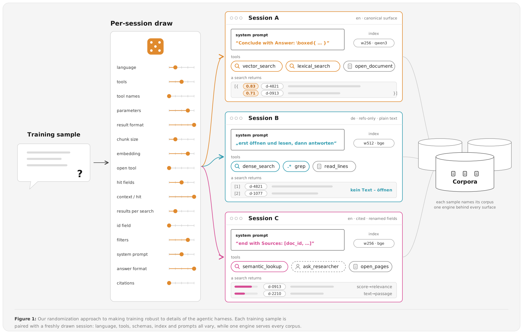
Our environment may be used in two ways. We may connect the environment to an existing “teacher” LLM—we use exclusively permissively licensed open-weight LLMs. This gives full “conversations” or “rollouts” on the basis of the environment, which may be used in the SFT phase of model-training, to “warm up” the model, ready for further refinement. In a second stage, “reinforcement learning” we may deploy the environment in the training environment, so that the latest version of Kolibri in training, may “attempt” to solve tasks. On the basis of the known correct answer, we may provide either encouragement (“reward”) or discouragement (negative “reward) to the model.
Sensitivity to runtime data distributions and use-cases
The LLM’s ability to leverage the agentic-harness, is not the only factor which affects the performance of the system at runtime. An additional key aspect of performance is the type of data which the application is deployed over—i.e. the content of the document corpora and data available to the LLM through its tools.
Many aspects of data can affect performance:
- Domain of the data (is it reflected by the pre-training distribution?)
- Surface aspects of the text (does is contain html/ tables/ etc. or other “difficult” data forms)
- Understanding how to deal with completely new data
- Contradictory or versioned data
- How closely irrelevant information in the text (distractors) is interleaved with the relevant information
Take the domain of the data, for example. A minimum of general knowledge is required for good performance in the RAG case. In the trace below, you can see that in order for the LLM to know which searches to fire off, to troubleshoot the user’s problem, it must understand the nature of problem, and the likely way this problem may be connected with the contents of the documentation, via search:
Since it turned cold, our Calvera AWP-12 heat pump switches on and off every few minutes. Is it broken?
Short on/off bursts are “short-cycling”. Three common causes: defrost cycles in cold, humid air; too little water in the heating circuit when zones are closed; a switching hysteresis set too narrow. The user’s words (“on and off”, “turned cold”) contain none of these terms, so the searches must use them. First, find out how the unit records why it stopped.
keyword_search("AWP-12 operating log compressor stop reason", corpus=manuals, k=5)
- AWP-12 Service Manual §5.2 Event Log (menu 4.7), p. 38 “…stop codes: D01 defrost, F12 low flow, H03 setpoint reached…”
The log tells the causes apart. Look up each one using the manual’s own terms.
semantic_search("frequent defrost cycles at low outdoor temperature and high
              humidity", corpus=manuals, k=3)
keyword_search("AWP-12 minimum water volume buffer tank", corpus=manuals, k=3)
keyword_search("AWP-12 hysteresis parameter", corpus=manuals, k=3)
- Installation Guide §3.4 Defrost Operation, p. 21 “…up to 3 defrost cycles per hour below 3 °C is normal…”
- Installation Guide §2.6 Hydraulics, p. 14 “…minimum system volume 60 l; below this, install a buffer tank…”
- Service Manual §6.1 Parameter P21, p. 44 “…switching hysteresis, default 2 K, range 1–6 K…”
All three causes have documentation. Send the user to the event log first, and give one fix for each stop code.
Probably not broken. Check the event log (menu 4.7, Service Manual p. 38) and see which stop code appears:
- D01 (defrost): up to 3 cycles per hour below 3 °C is normal (Installation Guide p. 21).
- H03 (setpoint reached) with many zones closed: the circuit may hold less than the 60 l minimum. Open more zones or add a buffer tank (p. 14).
- H03 with all zones open: widen the hysteresis, parameter P21, from 2 K to 4 K (Service Manual p. 44).
Sources: AWP-12 Service Manual pp. 38, 44 · Installation Guide pp. 14, 21
If we are able to train with a data distribution which correctly reflects the distribution of the data during production, then we are likely to perform better, than simply training on generic distributions. For Kolibri, the means we would like the peculiarities of the data we see at our customers to be reflected in the training distribution. However—we need to respect the key sovereign constraint—we cannot train with customer data.
In the next section we describe how we achieve this familiarity, without exposing Kolibri to customer data during training.
Training data distribution using synthetic task distributions
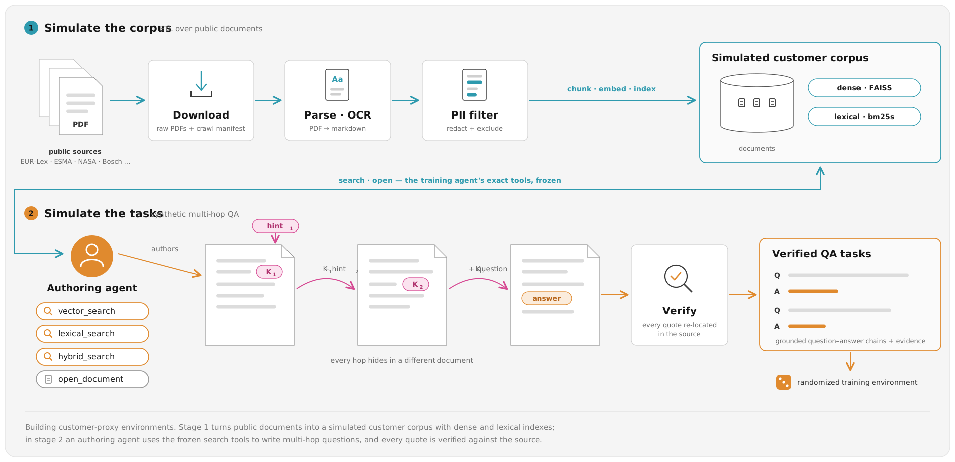
While building a workaround to the key sovereign constraint, we designed industry specific training data mixes to be used in our randomised training-harness setup; our models should be trained to become performant using data from technical, specific document distributions, in particular with a focus on German sources as well as English, in combination with a given harness. Here we were guided by the findings outlined by a team at Chroma.
To set up industry training data, we curate permissively licensed data from the open web. These corpora are chosen to reflect the distributions in our current and projected customer base; they include hardware documentation, open legal corpora and law listings, technical data sheets, economic data and descriptions and more. We then treat the data from each source as we do in production; it is ingested in preparation for various configurations of a RAG application. That means applying our pre-processing pipeline (ETL, chunking, filtering) with a variety of hyper-parameters, various embedding models, and agentic harnesses.
This preparation is succeeded by a second step, in which we generate tasks using synthetic generation which might plausibly have been posed by a human user. This is a workaround for the fact that we lack true gold-labels for these corpora.
Deploying industry specific environments inside training environments
Equipped with an environment which realises agentic-harnesses, and tasks over a range of corpora, we are faced with the challenge to shoe-horn this setup inside the training environment. The difficulty here is delivering our system into a larger system designed to learn the full gamut of skills from coding, to agentic tool calling through to hallucination reduction. As new skills are added to the training mix, we have to take care to avoid infrastructure bloat, which will lead to degradation in training throughput and model performance.
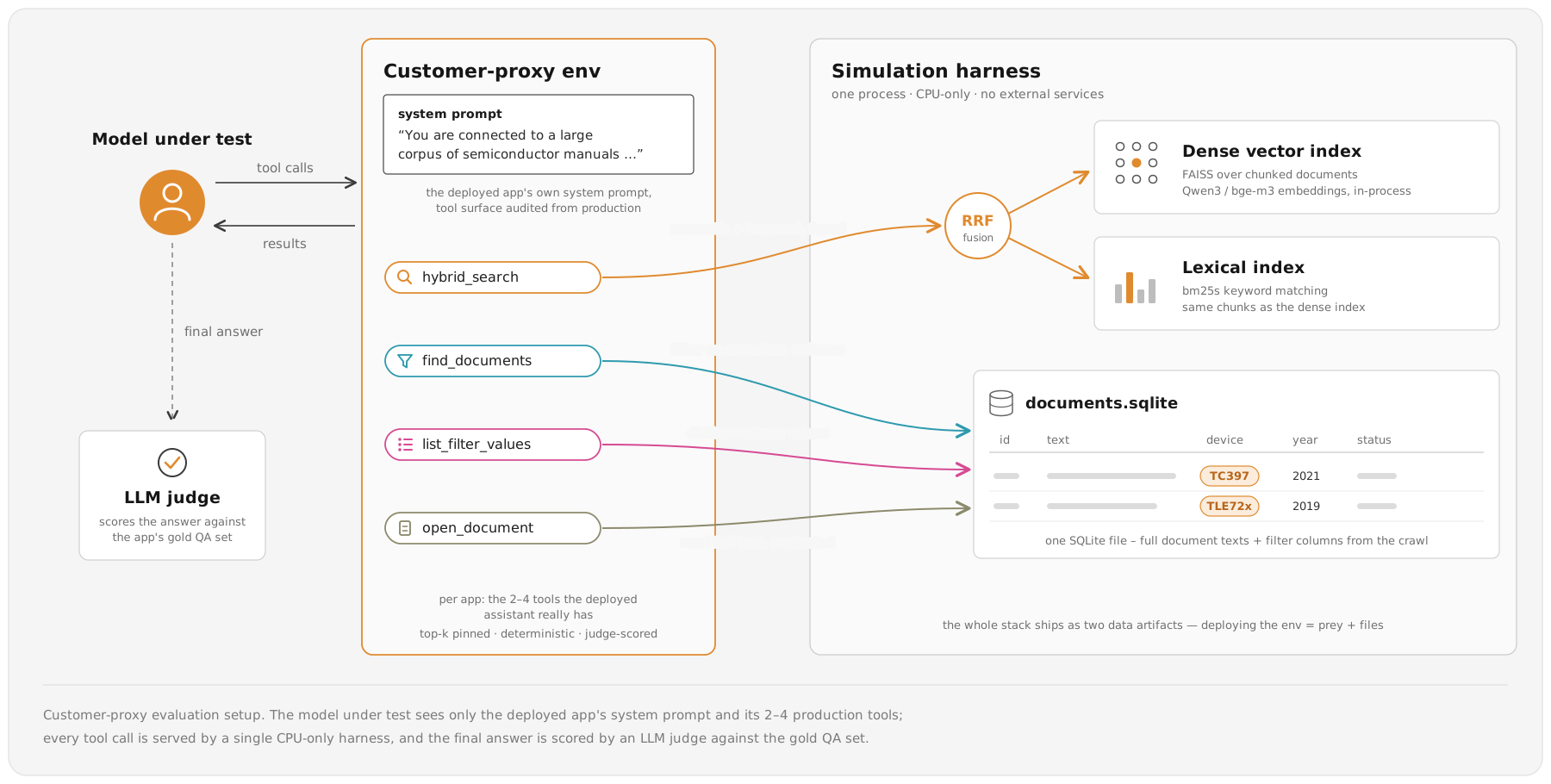
Our solution here was to make sure that the tool surface experienced by the model is “isomorphic” to the tool surface delivered to the model at inference/production, without transporting databases, authentication and a plethora of additional services into the training environment. Due to the fact that the tasks we are dealing with are read-only, we were at liberty to provide very lightweight and in-process simplifications of the production environments, without changing the model contract, in terms of the specification of the tool calls and APIs provided to the model. As a small indication of what this means, here are a few transformations we found expedient:
- Production database → SQLite
- Vector database → in-process static vector-index (FAISS)
- Grepping over large directories → post-processing results from a lexical index
Agentic and industry-specific benchmarks
In order to assess how well Kolibri generalises to mission critical use-cases, we built industry specific benchmarks. These are concrete realisations (no randomisation) of our environment using (a) the exact harness in use at one of our industry use-cases (b) either the exact corpus (for open corpora) or a corpus closely reflecting the type of data of interest in the use-case (c) either synthetic or expert provided gold-labelled task sets (no user data). We labelled these industry specific benchmarks, since they are the closest we can get to testing Kolibri on the use-case directly.
In addition to the industry-specific benchmarks, we maintained two additional benchmarks, based on publicly available corpora. The first was the test split of the MuSiQue data set; MuSiQue is a set of tasks which must be solved by multi-hop reasoning and information retrieval over an open-knowledge base. We cleaned and filtered the data, so that all questions posed are, in principle, answerable. The second benchmark was a portion of the industry specific training data, held out from training for evaluation purposes. We refer to this benchmark as Honeypot.
Training methods, iteration and incremental results
We post-trained Kolibri with supervised fine-tuning (SFT) followed by reinforcement learning (RL). We didn't have the compute for a full grid of controlled ablations. Instead, here is the sequence of experiments we ran, what each one taught us, and the few head-to-head comparisons that pin down where the gains came from. All accuracies in this section are judged by an LLM.
Step 1: Does the environment teach anything?
We started with a sanity check on a 30B model. We fixed the harness to the one used in evaluation and trained for 300 RL steps on general-knowledge multi-hop questions over an open knowledge base. MuSiQue accuracy rose by more than ten points, and the model learned to answer in fewer searches (7.6 down to about 5). With harness randomisation switched on, starting from a different checkpoint, the gain was the same size, and the model used about a fifth of the tokens per question. The industry-specific benchmarks, however, barely moved. General multi-hop skill was not carrying over to customer-style documents.
Step 2: Add industry-specific training data
We ran three 200-step ablations from the same Kolibri Origin checkpoint:
- Vertical-specific data alone: Honeypot more than doubled and the semiconductor benchmark nearly doubled from a low base. The other industry-specific benchmarks stayed within noise.
- General knowledge tasks alone: Honeypot fell below its starting point.
- The two mixed at equal weight: most of the Honeypot gain survived, and this run had the best MuSiQue score.
A large part of the Honeypot gain came simply from learning to stay within the 64K context window: context overflows dropped from 42% to 0.7%.
Step 3: Move to a bigger model
Once we added the environment to the main RL mix, typically for 500 to 2,000 steps, the hardest industry-specific benchmarks still lagged. The rollout traces showed why: the model overflowed its context and filled it with unnecessary searches. A longer context and stronger reasoning looked like the fix, so we moved to the 78B (3.4B active) architecture. To get a clean reference point, we first trained it for 1,000 RL steps on the full production mix without retrieval. On MuSiQue that model landed roughly on par with our earlier 30B releases. Adding the retrieval environment at just 3% of the mix lifted MuSiQue by well over ten points within a few hundred steps.
Over the following weeks we hill-climbed on the full mix. We adjusted the environment's weight, added tools and parameter ranges, and diagnosed failures from the industry specific benchmark rollouts, while checking that reasoning, coding and math didn't regress. As Figure 4 shows, we observed consistent improvement of all industry specific benchmarks in September.
Step 4: Feed the environment back into SFT
Using the same seed questions, we ran a strong teacher model through the environment. We kept only the rollouts that were correct, grounded in retrieved text and cleanly terminated, which gave about 16,500 gold agentic traces. Their effect was at least as large as RL's:
- With the RL recipe held fixed, training on the traces added 10–15 points on MuSiQue.
- The retrieval environment then added another 8–13 points on top of either starting point.
- Together, the two account for roughly 25 of the 30-point gap between our earliest 78B runs and the first production checkpoints.
On Honeypot, the traces drove most of the early gain and the environment added 5–8 points more. The industry-specific benchmarks were flat until a new SFT checkpoint with the traces arrived, then rose. By the end, the SFT checkpoint alone, before any RL, scored higher on MuSiQue than any of our 30B models.
Step 5: A better reward
Finally, we replaced the token-F1 reward with an LLM-as-a-judge reward, using the policy model itself as the judge so it needed no extra GPUs. In a four-way, 200-step comparison, judge-based rewards beat F1 by four to six points on MuSiQue. The improvement came from fewer wrong answers at the same number of turns. On Honeypot, every variant landed at the same score. There, the gain over the starting checkpoint came from learning to manage context, not from the choice of reward. Partial-credit and abstention rewards added nothing over a simple correct-or-incorrect judge, so that became our production default.
- Automotive supplier 0.72 → 0.99
- Semiconductors 0.35 → 0.80
- German public sector 0.54 → 0.75
- Industrial drive technology 0.31 → 0.60
- Aerospace 0.14 → 0.59
- one checkpoint, one eval
- mean of that day
- Kolibri Origin
- Kolibri
Final results
Figure 5 displays the final results on the released Kolibri model against various baselines. We tested Kolibri on seven benchmarks: MuSiQue, Honeypot, and the five industry specific benchmarks covering semiconductors, the German public sector, aerospace, automotive suppliers and industrial drive technology. We compared it with some of the strongest open-weight mixture-of-experts models around.
All baselines ran inside the same harness as Kolibri: the same system prompt, tool definitions, result-set sizes and 64K context budget, with no per-model prompt or tool tuning. Where a model exposes a reasoning-effort setting, we used its highest. The harness in each industry-specific benchmark is the one that use-case runs in production, so no model, Kolibri included, was evaluated in a harness adapted to it.
Kolibri comes out on top overall, with a mean score of 75.9. That puts it ahead of Qwen3.6-35B-A3B (71.1), Nemotron 3 Super (68.4) and Mistral Small 4 (62.6). It takes first place on four of the seven benchmarks and is within a few points of the leader on the other three. The standout is the automotive supplier task, where Kolibri scores 99.0.
What makes this interesting is efficiency. Kolibri has 78B parameters in total but activates only a small fraction per token. Nemotron 3 Super uses roughly four times as many active parameters and Mistral Small 4 nearly twice as many, and Kolibri beats both. Qwen3-Next 80B-A3B has nearly the same size and active-parameter budget, yet trails by a wide margin; its successor Qwen3.6-35B-A3B is a close second in the same harness, so the gap is the model, not the harness.
It's also a big step up from Kolibri Origin, our earlier and smaller 30B MoE model. The average score nearly doubles, from 39.3 to 75.9. The jumps are biggest on Honeypot (+55 points), Semiconductors (+45) and Aerospace (+45).
To be fair, the race is close in places. Qwen3.6-35B-A3B is right behind Kolibri on several of the industrial benchmarks and edges it out on Aerospace by just 0.1 points.
Across the whole suite, though, Kolibri gives the best results, and it does that with a fraction of the compute per token.
Show the numbers
| Benchmark | Kolibri | Kolibri Origin | Qwen3-Next 80B-A3B | Qwen3.6-35B-A3B | Nemotron 3 Super 120B-A12B | Mistral Small 4 119B-A6B |
|---|---|---|---|---|---|---|
| MuSiQue (cleaned) | 77.3 | 42.7 | 50.5 | 61.2 | 79.1 | 66.8 |
| Honeypot | 80.8 | 25.3 | 13.5 | 74.3 | 68.8 | 68.1 |
| Semiconductors | 80.4 | 35.3 | 41.2 | 79.4 | 69.6 | 62.7 |
| German public sector | 75.0 | 54.0 | 29.5 | 72.0 | 78.0 | 50.0 |
| Aerospace | 58.9 | 14.1 | 48.1 | 59.0 | 54.9 | 47.0 |
| Automotive supplier | 99.0 | 72.4 | 84.2 | 92.6 | 91.0 | 87.1 |
| Industrial drive technology | 60.0 | 31.4 | 32.7 | 59.5 | 37.3 | 56.8 |
| Benchmark | Kolibri | Qwen3.6-35B-A3B | Nemotron 3 Super | Mistral Small 4 | Qwen3-Next 80B-A3B | Kolibri Origin |
|---|---|---|---|---|---|---|
| MuSiQue (cleaned) | 77.3 | 61.2 | 79.1 | 66.8 | 50.5 | 42.7 |
| Honeypot | 80.8 | 74.3 | 68.8 | 68.1 | 13.5 | 25.3 |
| Semiconductors | 80.4 | 79.4 | 69.6 | 62.7 | 41.2 | 35.3 |
| German public sector | 75.0 | 72.0 | 78.0 | 50.0 | 29.5 | 54.0 |
| Aerospace | 58.9 | 59.0 | 54.9 | 47.0 | 48.1 | 14.1 |
| Automotive supplier | 99.0 | 92.6 | 91.0 | 87.1 | 84.2 | 72.4 |
| Industrial drive technology | 60.0 | 59.5 | 37.3 | 56.8 | 32.7 | 31.4 |
| Mean | 75.9 | 71.1 | 68.4 | 62.6 | 42.8 | 39.3 |
Discussion
We successfully trained Kolibri to achieve RAG performance outclassing models in its weight class and above, for agentic-RAG applications, and in particular applications relevant to our customers. We followed an analytical and explorative approach; we analysed the feature set and data distributions expected in our use-cases, built environments to simulate these conditions, and used an explorative empirical approach based on feedback from training, to optimise the environment in tandem with the LLM’s core abilities.
To fully understand the factors affecting performance and leading to our strong performance, careful ablations are necessary, which lay outside the scope of our ambitious timeline and computational constraints. In addition, caution should be exercised when interpreting “specialised performance” increases, in particular when considering the robustness of the solution to aberrations in the inference setup—this is why the randomisation aspect of our environment was important for serving customers going forward. Ultimately, the performance metric which cannot lie is continuous monitoring of the solution in live production customer deployments. We believe, however, that by carefully decomposing our customer requirements and use-cases into component parts, and simulating the harness, corpus and task axes separately, the model has every chance to adapt well to changing data, requirements and harnesses.
Conclusion
In this post, we discussed the challenges and potential solutions in specialising language models for sovereign data-backed LLM deployments. Our initial approach has led to effective optimisation of our internal models, allowing them to compete at a weight class above their own on key agentic-RAG metrics, both open benchmarks and industry specific metrics. Future model releases will build on this approach, extending our findings to a wider class of tasks and use-cases.
Acknowledgements
The work described in this post was a collaborative effort between Duncan Blythe, Till Speicher, Alexei Zacharov and Pranav Ragupathy, together with research, engineering and customer teams at Aleph-Alpha. Many thanks to all of the great people who contributed to helping push Kolibri to the Pareto frontier of agentic RAG performance, and the amazing support throughout the company.